
Quick Look
Grade Level: 11 (10-12)
Time Required: 45 minutes
Lesson Dependency: None
Subject Areas: Computer Science, Science and Technology
Summary
Dive into the rapidly emerging world of machine learning, where students come to understand the first attempts at developing the perceptron model—a simplified model of a biological neuron. Students also learn about the logic of the perceptron model and its limitations, which led to the development of multi-layer networks.
Engineering Connection
Machine learning is the process by which a computer is able to improve its own performance by continuously incorporating new data into an existing statistical model.
Computer scientists use machine learning to automate the process of data analysis in a variety of industries. In the financial sector, engineers apply principles of machine learning to engineer systems that can gain insights into complex data sets to prevent fraud. Healthcare professionals can use machine learning to help improve diagnoses and treatments. Computer scientists must understand the logic of the particular machine learning model and mathematics involved in machine learning in order to choose the appropriate model and parameters.
In the associated activity, Computer Simulation of an Artificial Neural Network, students play the role of the computer scientist by comparing the logic of two machine learning models including their strengths and weaknesses.
Learning Objectives
After this lesson, students should be able to:
- Define machine learning.
- List examples of how machine learning is used in different industries.
- Describe the process of using a machine learning model.
- Describe how the perceptron model learns.
- Describe the major weakness of the perceptron and how engineers overcome this weakness.
Educational Standards
Each Teach Engineering lesson or activity is correlated to one or more K-12 science,
technology, engineering or math (STEM) educational standards.
All 100,000+ K-12 STEM standards covered in Teach Engineering are collected, maintained and packaged by the Achievement Standards Network (ASN),
a project of D2L (www.achievementstandards.org).
In the ASN, standards are hierarchically structured: first by source; e.g., by state; within source by type; e.g., science or mathematics;
within type by subtype, then by grade, etc.
Each Teach Engineering lesson or activity is correlated to one or more K-12 science, technology, engineering or math (STEM) educational standards.
All 100,000+ K-12 STEM standards covered in Teach Engineering are collected, maintained and packaged by the Achievement Standards Network (ASN), a project of D2L (www.achievementstandards.org).
In the ASN, standards are hierarchically structured: first by source; e.g., by state; within source by type; e.g., science or mathematics; within type by subtype, then by grade, etc.
NGSS: Next Generation Science Standards - Science
-
Analyze data using tools, technologies, and/or models (e.g., computational, mathematical) in order to make valid and reliable scientific claims or determine an optimal design solution.
(Grades 9 - 12)
More Details
Do you agree with this alignment?
-
Models (e.g., physical, mathematical, computer models) can be used to simulate systems and interactions—including energy, matter, and information flows—within and between systems at different scales.
(Grades 9 - 12)
More Details
Do you agree with this alignment?
Common Core State Standards - Math
-
Summarize, represent, and interpret data on two categorical and quantitative variables
(Grades
9 -
12)
More Details
Do you agree with this alignment?
International Technology and Engineering Educators Association - Technology
-
Students will develop an understanding of the characteristics and scope of technology.
(Grades
K -
12)
More Details
Do you agree with this alignment?
State Standards
Michigan - Math
-
Summarize, represent, and interpret data on two categorical and quantitative variables
(Grades
9 -
12)
More Details
Do you agree with this alignment?
Worksheets and Attachments
Visit [www.teachengineering.org/lessons/view/mis-2484-machine-learning-perceptron-modeling-lesson] to print or download.Pre-Req Knowledge
Strong math skills and a familiarity with boolean logic is helpful.
Introduction/Motivation
Has anyone heard of machine learning? What is it? Can anyone give a definition? (Expect answers to cite artificial intelligence as an example; have the first three slides from the PowerPoint Presentation ready to show the definition of machine learning as a subset of artificial intelligence.)
Do you have a smartphone? Do you use voice-to-text? Did you know that your smartphone uses machine learning to better understand your specific voice? Machine learning is also used in many other industries as well. (Show slide 4 showing uses of machine learning).
Does anyone know when machine learning was first designed? (Expect a wide range of answers and maybe even 1990’s or 2000’s). Did you know that this was thought about in the 1940s with one of the earliest designs coming in 1958?
So, just how does a machine learn? Today we will look at the basic logic a machine learning model uses and in particular we will look at the perceptron model, the first attempt at machine learning. It is a type of artificial neural network (ANN or neural network for short). The artificial neural network is modeled after the human brain. A neuron takes an input signal, processes it and “fires.” In other words, it passes the input signal as an output to the next neuron. Neurons are a part of a much larger system of neurons to help make decisions. As an example, when making a decision to wear a coat, one neuron could “ask”, so to speak, “is it below 60 degrees?” If yes, this neuron returns an output of true and if not, this neuron returns an output of false. The brain is comprised of many neurons and of course there are other decisions that may be factored in such as “is it raining?” Neurons compute these decisions in layers and continue to pass the outputs down from layer to layer. Once all of these decisions have been made and all of the outputs have been passed along, the decision as to whether or not to wear a coat would be made if the overall sum of all the outputs is greater than some threshold number. (look at slides 5 and 6 together; slide 5 is the general case and may be skipped at your discretion, slide 6 is a simple example of a neural network handling the decision on whether or not to attend the high school football game on Friday.)
Let’s talk about setting up the conditions which will produce an output of 1. We will need to start with an understanding of some basic logic functions. We will only look at questions which can be answered as yes/no or true/false. We call these Boolean data types. This means we can represent these as 0 for no (or false) and 1 for yes (or true). (The teacher may want to keep a running list of the engineering vocabulary on a board).
Let’s begin with the “OR” function. This means that if either condition is true, the output is 1. (Show slide 7 of the OR function and talk through the logic. Make sure the students understand this and then have the students take 1-2 minutes to complete the challenge on the slide, which is to think about all of the possible combinations of inputs and their sum. Answer key is provided on the next slide, slide 8.)
Let’s make sure you understand something which is called set notation. (pointing to slide 7)
“y ∈ {0,1}” ” is read “y is an element of the set (0,1)” and just means y can be 0 or 1. The greek letter you see is an epsilon. It looks like the letter “e” so you can think of it as an e for “element.”
Now, take a few minutes to complete the table on the screen. You should have 4 columns just as it shows on this slide here. The x1 + x2 column will be used for something in just a few minutes, but this is just the sum of the first two columns. How many possible combinations of inputs can you have? If x1 is 1, x2 could be 1 or ____? (answer is 0). Think about the possibilities and complete the table.
(Go around the room to check understanding. After this, go to the “OR Functions Answer” slide 8 after 1-2 minutes and talk through the three combinations which produce an output of 1).
Now look at the table of answers. We can actually treat these sets of inputs as points and plot them on a graph. (Show slide 9, OR Function A Geometric View) We will treat x1 as the x-axis and x2 as the y-axis. This gives us a nice visual of the combinations of inputs which produce a 0 or 1. In addition to plotting these points, a boundary line is drawn. This boundary line splits the data into 2 groups. Group 1 contains all of the points which produce a 0. In this case, there is just one point (0,0). Group 2 are all of the points which produce an output of 1. These are the points on the boundary line or above. We call this concept linear separable. This means there is a line which can divide up our points in this way. (Slides 22-25 at the end of the slideshow contain a short exercise about linear separability. This could be done prior to talking about the OR Geometric view or after or can be skipped at teacher discretion).
(Show slide 10.) Let’s move on to the AND function. Just like we did for the OR function, let’s come up with all of the possibilities for the values of the inputs which will be the same as before. What will change is the last 2 columns. We want to calculate the sum like we did before and identify which input combinations will produce an output of 1. (Go around the room to help and check understanding. Give the students 1-2 minutes to complete the challenge shown on the slide, then show the answers on slide 11 and talk through them).
(Move on to slide 12. Take 1-2 minutes and have the students plot the points and boundary line for the AND function on their own paper. Graphing this may prove difficult for the students.)
Now plot all of the possible points from our table just like we did for the OR function. Does a boundary line exist? And if so, sketch it in.
(Go to slide 13 which shows the answer) The only possible combination of inputs which satisfy the AND condition and produce an output of 1 is (1,1). The sum of this one combination is 2 so the threshold in this case is 2. Notice the boundary line would have intercepts at (0,2) and (2,0) but 2 is not a possible input.
(Move on to the XOR slide, slide 14). Now let’s talk about one last logical function, XOR. XOR is short for “Exclusive OR.” This is like OR but the case of both is not accepted. So, XOR is one or the other, but not both. As we did before, complete the table for the XOR function. (Give the students 1-2 minutes to complete the challenge shown on the slide, go around and check for understanding. Then, show the answer on slide 15.)
The point (1,1) does not produce an output of 1. Is this linear separable? Let’s review what that means: Can you draw a single line which will separate the 1 outputs and 0 outputs? (Show slide 16. Students may think they can draw a line connecting (0,0) and (1,1) but these points do not belong in the same group and therefore would not be allowed on the same line. Give a minute or two for discussion.)
As it turns out, XOR is not linear separable since the best candidate for a line, the one connecting (0,0) and (1,1) does not actually separate outputs of 0 and 1. These points belong in two different groups and therefore cannot be on the same line.
Let’s go back to our simple model of whether or not I will attend the football game on Friday (A duplicate slide is inserted as slide 17 as a visual). As I said, this example is very simplistic as it doesn’t give all of the factors that would go into making this decision. Also, let’s discuss the importance of each one of these decisions. Are these decisions treated the same or differently in this scenario? (Wait for student responses and expect a little discussion. A good discussion about mathematical modeling and assumptions can be had as well). This model treats these decisions as being equal, but do you think this is realistic? (Hopefully students will add to the discussion and state that some factors may be more important than others).
(Go to the “Using Weights” slide, slide 18) Here you can see how the importance of decisions can be represented by giving a particular weight to each input.
(Go to the “Using Weights Example” slide, slide 19)
Let’s say we have a situation with 3 inputs and the weights shown here. And let’s say this neuron will fire if the threshold is 0.5. Notice in this case that the neuron does result in a 1 even though 2 of the 3 inputs are 0. This is because the weight given to x1 is larger than the weights given to the other two inputs.
Perceptron Model
As mentioned earlier, one of the earliest models of the biological neuron is the perceptron. The perceptron model works in a very similar way to what you see on this slide using the weights. But how does it learn? Any machine learning model requires training data. This is the data given to the model where the output is already known. The model will start off by picking random weights. It will then go through a lot of data and see if it can establish a rule for all cases. If we go back to our geometric representations, the perceptron model will try to find a combination of weights that will produce a line that separates the outputs of 0 and 1 just like we talked about before.
One major difference is that the threshold value is actually used as an input. This is done by simple algebra.
w1x1 + w2x2 + w3x3 ≥ θ
or w1x1 + w2x2 + w3x3 - θ ≥ 0
(You may want to show this on the board or use the “Perceptron Model” slide, slide 20)
Before we talked about the threshold value: the value for which it would take to produce an output of 1. The bias is the same idea only it is moved to the other side of the inequality in order to be able to control it when going through the machine learning process.
(Move to the next slide “Perceptron Model Workflow,” slide 21. You may want to have students take turns reading each step)
Take some time to look over this workflow. The next major difference is presented here and that is the learning rate. This is a parameter that is used to control how much the weights are changed when the model is going through the training process. (Some questions may be asked about the bias. This can be explained in a few ways and it may be helpful to explain the meaning as it relates to the common, everyday definition of the word. Using the football game example, the bias may represent how much or how little of a football fan you are.)
Lesson Background and Concepts for Teachers
The lesson will give students a background of machine learning, particularly the perceptron model (Figure 1). The associated activity, Computer Simulation of an Artificial Neural Network, will have students use a simulation of the Perceptron model on the Netlogo platform and discover a significant limitation of this model and then move on to run simulations using the multi-layer Perceptron model.

Background
A very rudimentary and simple explanation of how biological neurons work is helpful to both the teacher and the student. Fundamentally, a neuron takes an input signal, processes it and “fires.” In other words, it passes the input signal as an output to the next neuron. Neurons can be thought of as a part of a larger system of neurons to help make decisions. As an example, when making a decision to wear a coat, one neuron could be the “is it below 60 degrees?” neuron. If yes, this neuron returns an output of true and if not, this neuron returns an output of false. The brain is comprised of many neurons and of course there are other decisions that may be factored in such as “Is it raining?” Neurons compute these decisions in layers and continue to pass the outputs down from layer to layer. Once all of these decisions have been made and all of the outputs have been passed along, the decision as to whether or not to wear a coat would be made if the overall sum of all the outputs is greater than some threshold number.
Keep in mind that the human brain has approximately 1011 neurons, so it should be easy to see how complex this can quickly become.
The first computational model of a biological neuron was proposed by McCulloch and Pitts in 1943. The McCulloch-Pitts artificial neuron allowed boolean values (e.g. true = 1 or false = 0) and worked very similar to the description above.
, x_(2 ,) x_(3 )on the left and an output of y on the right. In the middle of the neuron is the threshold value of theta.")
Figure 2 shows that for each input, x1, x2, x3 the output of y will be 1 if x1 + x2 + x3 ≥ θ. If x1 + x2 + x3 < θ, then the output of y = 0.
Another simple example can be seen in the decision to go see the high school football team play. 3 inputs could be set up as:
x1 = Does the team have a good chance of winning?
x2 = Is the weather nice?
x3 = Is it a home game?
Let’s say the decision to attend the game will be made if the sum of the inputs ≥ 2. e.g. in this case, θ = 2.
Please keep in mind these are simple examples with only 3 inputs. In reality, there could be hundreds or thousands of inputs. The simplicity can be used to discuss how mathematical models make assumptions and are simpler than the real world.
In order to understand the machine learning models in this lesson, it will be important to understand a few logical functions.
AND function
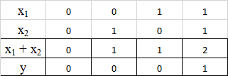
Figure 3 shows the “And” function with 2 inputs. This neuron is to only fire if both x1 = 1 and x2 = 1. Another way of saying this is to say that the threshold value θ = 2.
Table 1 below shows the 4 possible combinations of values for inputs along with the sum of the input values and the resulting output, y. The column on the far right represents the only scenario where both x1 = 1 and x2 = 1 which is the definition of the “And” function. Therefore, 2 should be the threshold value θ.
It is important to understand the geometric representation of this. The simulation in the Computer Simulation of an Artificial Neural Network communicates the rule the model has learned through the training using this geometric interpretation. Figure 4 is a graph of the above 4 scenarios with each dimension representing the inputs.
 to (2,0) and passes through (1,1).")
You will also notice the graph contains a boundary line. Any points on or above this boundary line will produce an output of 1. The only such possible point is the point (1,1). You can look to see that the other 3 points are below the boundary line. This concept is known as linear separability. Linear separable means that there is a line that can separate the inputs so all inputs resulting in an output of 1 are on one side of the line and all inputs resulting in 0 are on the other.
OR Function
, x_(2 ) on the left and an output of y on the right which can be 0 or 1.. In the middle of the neuron is the threshold value of 1.")
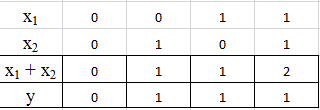
Figure 5 shows the “OR” function with 2 inputs. This neuron is to only fire if either x1 = 1, x2 = 1 or both = 1. The threshold value θ = 1 in this case (see the table below).
Table 2 below shows the 4 possible combinations of values for inputs along with the sum of the input values and the resulting output, y. You can see columns 2,3 and 4 represent the scenarios x1 = 1 OR x2 =1 (or both) which is the definition of the “OR” function. Therefore, 1 should be the threshold value θ.
Similar to what was done above with the “AND” function, the “OR” function can be represented geometrically. See Figure 6.
as the x-axis and x_(2 ) as the y-axis. The boundary line is graphed going from the points (0,1) to (1,0) and passes below (1,1). The equation for the threshold is shown as x_(1 )+x_(2 ) = θ= 1.")
The boundary line in this case is shown. Any point on or above the line produces an output of 1 since the sum of the inputs are greater than or equal to the threshold value θ = 1. For the “OR” function, (0,1) and (1,0) are on the line and (1,1) is above the line so these are the three scenarios which will produce an output of y = 1. The point (0,0) is the only scenario which produces an output of 0 and is represented geometrically by the fact that it is below the boundary line.
XOR
“XOR” is the case of one or the other, but not both. This function is NOT linearly separable which means the McCulloch-Pitts and Perceptron models will not be useful. XOR produces an output of 1 in the cases of (0,1) and (1,0). In looking at the geometric representation of the “OR” function, hopefully you can tell that a single line cannot separate the two sets of inputs resulting in 1 and the two sets of outputs resulting in 0, which are (0,0) and (1,1).
Perceptron
The Perceptron was introduced in 1958 by American Psychologist Frank Rosenblatt and refined by Minsky and Papert in 1969. The Perceptron overcomes some of the limitations of the McCulloch-Pitts model.
The basic structure of the Perceptron model is similar to the McCulloch-Pitts model, however there are two important differences.

In Figure 7, you can see the overall idea is the same except for two important differences:
- The inputs to the function are weighted as represented by wn.
- The threshold value of θ, is actually represented as a weight to an input of 1. Because it is an input it is represented as -θ. This might seem tricky, but it is just because it is moved to the other side of the inequality. Remember, the neuron fires when the sum of the inputs are greater than or equal to some threshold value θ. In other words:
w1x1 + w2x2 + w3x3 ≥ θ
or w1x1 + w2x2 + w3x3 - θ ≥ 0
- θ in this case can be interpreted to be a bias. In the example about watching the high school football game, this might represent how much the person likes football.
There are two major improvements of the perceptron over the McCulloch-Pitts model:
- The weights, including -θ, can be learned over time.
- The model can accept real numbers, not just boolean values.
These two improvements make this model more useful in real-world applications.
A major limitation still exists though. The Perceptron can only be used for functions that are linearly separable, like the “AND” and “OR” cases above, but not the “XOR” case.
How the model learns
Machine learning requires the model to be trained on training data. The model is given data where the actual outcome is known. The model calculates its output and then compares this output to the actual output to make adjustments. The perceptron is no different. Initially, the perceptron model is given a set of weights including the bias. The perceptron uses training data to calculate a weighted-sum using the weights and the values of the inputs to check whether or not the model outcome matches the actual outcome. If the model produces an incorrect result, an adjustment is made. This adjustment uses the error of the model and also a value called the learning rate. The learning rate is chosen in the beginning of the training and helps control how much the bias and the weights are changed for each adjustment. This process is repeated over and over until the model is trained.
Multi-layer Perceptron
A multi-layer perceptron is what it sounds like: it’s a network of more than one perceptron. Inputs are put into the first layer and then passed to the next layer and so on. Initially, it was thought that adding layers to the perceptron wouldn’t help overcome the issues of the single perceptron. It was later proven that a multi-layered perceptron will actually overcome the issue with the inability to learn the rule for “XOR.” There is an additional component to the multi-layer perceptron that helps make this work: as the inputs go from layer to layer, they pass through a sigmoid function. This sigmoid function is used in order to give the system more flexibility to its outputs.
A great example illustrates the reason for using such a function. Think about the problem of deciding whether or not to watch a movie based on a critic’s rating of 50% or higher. What will the decision be if the rating is 51%? Yes! What will be the decision if the rating is 49%? No!
This decision may seem a bit harsh, after all, is there really that much of a difference in the quality of a movie between a rating of 49% and 51%? Think about what this would look like mathematically. This would look like a step function where the output =0 for ratings between 0 and 0.49. At 0.5, the output jumps to 1. See Figure 8.

By passing the output through a sigmoid function (such as tanh), this transition becomes much smoother and allows for more flexibility in the outputs. A visual comparison is shown below where the red curve is the sigmoid function shown in Figure 9:

A natural question in looking at this graph may be asked by noticing that the values represented by the red curve are less than 1 when the threshold value is between .5 and 1. Because the original input is being passed through the sigmoid function, the output no longer represents the usual output (a binary value of either 0 or 1), it is a real number between 0 and 1. This actually corresponds to a probability. The Machine Learning algorithm will use this probability to decide whether the output should be 0 or 1. Ultimately, students just need to be made aware that the purpose of the sigmoid function is to smooth out the transition between 0 and 1.
In the Computer Simulation of an Artificial Neural Network, students will go through the NetLogo simulation of the perceptron for the case of “AND” as well as “OR.” Students will see the perceptron model quickly learning the weights and the rule (the boundary line in our geometric representations). As discussed here, the rule for “XOR” can never be learned by the perceptron model since it is not linearly separable.
At this point in the activity, students will move on to the multi-layer model and see how adding a layer can overcome the limitation of the single perceptron.
Two very helpful resources which should be read in order are listed below. These articles outline the history of the modeling of the neuron and how the perceptron model was built to overcome the limitations of the first attempt:
McCulloch-Pitts Neuron — Mankind’s First Mathematical Model Of A Biological Neuron
Perceptron: The Artificial Neuron (An Essential Upgrade To The McCulloch-Pitts Neuron)
Two other helpful resources come from the descriptions of the simulation in the Netlogo library. They contain more information on how the simulations work on Netlogo and a more in-depth discussion of the mathematics behind the models:
Associated Activities
- Computer Simulation of an Artificial Neural Network - Students use the Netlogo platform to run simulations of a basic neural network called the perceptron.
Lesson Closure
“In this lesson, we covered some basic ideas of how a simple artificial neural network works. We defined the terms machine learning and artificial neural network and identified applications where these are used. We looked at boolean values and how the logic of machines work by understanding the “AND,” “OR,” and “XOR” functions. We studied two different artificial neural network models: the perceptron and the multi-layered perceptron to gain an understanding of the history of machine learning as well as the logic and mathematics involved in machine learning. We discussed how all machine learning models work using training data and the model’s error to make adjustments in order to learn.”
Vocabulary/Definitions
algorithm: Process or set of rules to be followed in calculations.
artificial neural network: A type of machine learning inspired by the structure of the human brain. These systems learn, not by being given explicit instructions, but by looking at samples of information.
Boolean data type: Data type with one of two possible values, often noted as true or false.
epoch: Complete run through all the training instances.
learning rate: Value used in machine learning to control how much of an adjustment is made to the parameters between attempts during the training phase.
linear separable: If two sets of points can be divided by a single line, these points are said to be linearly separable.
machine learning: The process by which a computer is able to improve its own performance by continuously incorporating new data into an existing statistical model.
sigmoid function: Type of function with an s-shaped curve.
step function: Function that increases or decreases abruptly from one constant value to another.
training data: In machine learning, training data is the data used to train the model. The outcome is known and used to check the model and calculate an error. This error is then used along with the learning rate to adjust the parameters of the model.
XOR: Exclusive; for example, one or the other, but not both.
Assessment
Pre-Lesson Assessment
Discussion: Have students share what they know about machine learning and see if they can come up with a definition. Have students identify areas where machine learning is used.
Post-Introduction Assessment
Assessment: After completing the introduction, have students complete the Post-Introduction Assessment.
Lesson Summary Assessment
Summary Assessment: After completing the lesson, have students complete the Lesson Summary Assessment.
Subscribe
Get the inside scoop on all things Teach Engineering such as new site features, curriculum updates, video releases, and more by signing up for our newsletter!More Curriculum Like This

High school students learn how engineers mathematically design roller coaster paths using the approach that a curved path can be approximated by a sequence of many short inclines. They apply basic calculus and the work-energy theorem for non-conservative forces to quantify the friction along a curve...

Learn the basics of the analysis of forces engineers perform at the truss joints to calculate the strength of a truss bridge known as the “method of joints.” Find the tensions and compressions to solve systems of linear equations where the size depends on the number of elements and nodes in the trus...

Students learn about the science and math that explain light behavior, which engineers have exploited to create sunglasses. They examine tinted and polarized lenses, learn about light polarization, transmission, reflection, intensity, attenuation, and how different mediums reduce the intensities of ...

Students learn about nondestructive testing, the use of the finite element method (systems of equations) and real-world impacts, and then conduct mini-activities to apply Maxwell’s equations, generate currents, create magnetic fields and solve a system of equations. They see the value of NDE and FEM...
References
Toward Data Science, Medium.com. https://towardsdatascience.com. Accessed 3/31/2020.
Rand, W. and Wilensky, U. NetLogo Artificial Neural Net - Perceptron model. Center for Connected Learning and Computer-Based Modeling, Northwestern University, 2006. http://ccl.northwestern.edu/netlogo/models/ArtificialNeuralNet-Perceptron. Accessed 3/31/2020. Rand, W. and Wilensky, U. NetLogo Artificial Neural Net - Perceptron model. Center for Connected Learning and Computer-Based Modeling, Northwestern University, 2006. http://ccl.northwestern.edu/netlogo/models/ArtificialNeuralNet-Perceptron. Accessed 3/31/2020.
Rand, W. and Wilensky, U. NetLogo Artificial Neural Net - Multilayer model. . Center for Connected Learning and Computer-Based Modeling, Northwestern University, 2006. http://ccl.northwestern.edu/netlogo/models/ArtificialNeuralNet-Multilayer. Accessed 3/31/2020.
Copyright
© 2020 by Regents of the University of Colorado; original © 2019 Michigan State University.Contributors
Chris Tyler, High School Math Teacher, Lansing, MISupporting Program
RET Program, College of Engineering, Michigan State UniversityAcknowledgements
This curriculum was developed through the Michigan State University College of Engineering NSF RET program under grant number CNS-1854985 under National Science Foundation. However, these contents do not necessarily represent the policies of the NSF, and you should not assume endorsement by the federal government.
Last modified: October 23, 2025
User Comments & Tips